SORT Function in Excel – how can I use this function in my spreadsheets? Watch the video to learn more
![]() This week’s hint and tip is on the SORT function in Excel. It looks at this function and how it can be used in spreadsheets. This isn’t covered specifically in our courses so we decided to do a hint and tip on it. We are going to go through it now below.
This week’s hint and tip is on the SORT function in Excel. It looks at this function and how it can be used in spreadsheets. This isn’t covered specifically in our courses so we decided to do a hint and tip on it. We are going to go through it now below.
What is the SORT Function?
The new SORT function covers functionality which you can perform using Data Sort. However where Data Sort re-sequences the original list, the SORT function gives the results of the sorted list on the same worksheet in a different place leaving the original list alone.
In the video we look at a simple 1 level SORT to see how the function works. In a future video and blog, we will look at the SORTBY function which allows multiple sorts.
Below is a picture of the list of data in the video and the SORT function in the formula bar.

The SORT Syntax
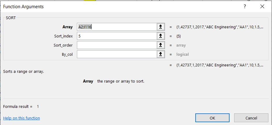
The syntax of the SORT function is below. We select an empty cell with its headings as per the original ones.

The Array is the range of data we wish to sort.
The Sort_index is the column number of that array that is the new sort sequence – in this case its column 5 the customer name.
The Sort_order defaults to 1 which refers to ascending and -1 is the choice for descending. There is no need to type in 1 for ascending.
By_col: default is False to sort by row which is what we wish to do. You can also sort by column. Again, no need to type in anything here.
This gives as you can see a new set of sorted data starting in cell K2.
The video below shows you how to use the SORT function in Excel. It goes through what this function does in the spreadsheet and how to use it.
Take a look below at the video to find out more and then try it out on your own computer!
We hope you have enjoyed this hint and tip on the SORT function in Excel. Why not take a look at our previous one on some useful features in Excel?
