
Excel Conditional Formatting with Dates – taking conditional formatting a step further in your spreadsheets
![]() This week’s hint and tip is on Excel conditional formatting with Dates. Conditional formatting is a very useful feature in Excel and being able to use it alongside dates can be very useful. This is covered in our Intermediate Excel training course but we also decided to do a hint and tip on it. We are going to go through it now below.
This week’s hint and tip is on Excel conditional formatting with Dates. Conditional formatting is a very useful feature in Excel and being able to use it alongside dates can be very useful. This is covered in our Intermediate Excel training course but we also decided to do a hint and tip on it. We are going to go through it now below.
Conditional Formatting with Dates
In this blog we shall look at a real-life example of how a company may manage using colour appliance tests which are due for re-testing. The background to this blog and video was born out of a recent question at a client site who asked about managing their testing procedure better.
The worksheet is attached for you to look at (further down in the post) but here is a screen print of it too.
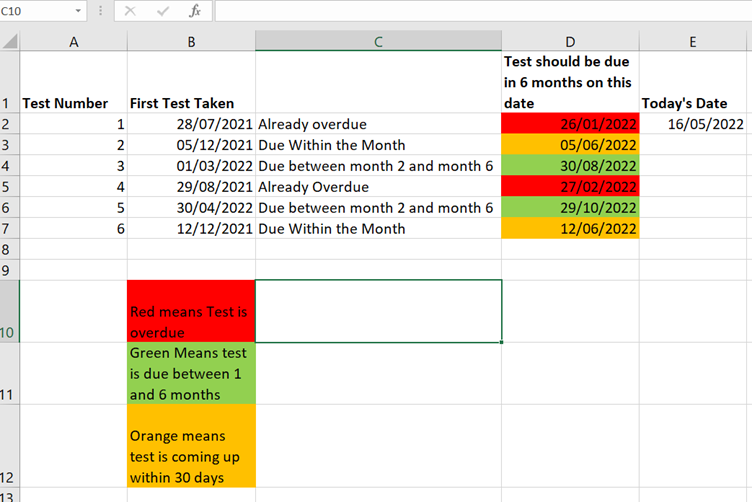
Effectively the first test took place on the date in column B. Note also today’s date was 16/05/2022 and 6 months after the first date there is a date in column D.
Effectively the colour chart at the bottom of the sheet explains what colour means what. To compose this we had to use Conditional Formatting using formulas.
Red Rule (Overdue)
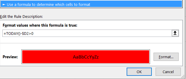
If today’s date is greater than the date of re-test its late!
Orange Rule (Due within the month)
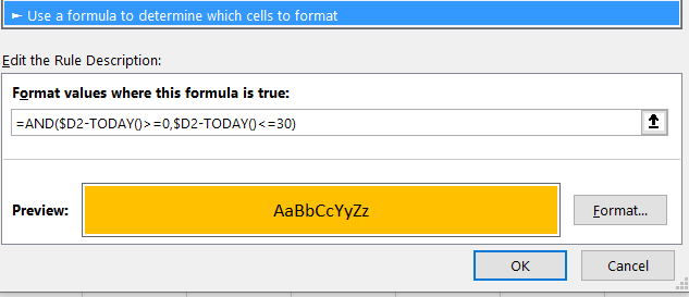
If the difference is only up to 30 days, then its due within the month. To compose this we used an AND function and in this function both conditions need to be true for it to turn orange.
Green Rule (Due between month 2 and month 6)
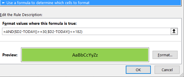
Here again an AND function is used and the difference between due test date and today is between 30 and 180 days i.e. month 2 and month 6 to turn green.
We cover other elements of conditional formatting in our Excel series of courses in both our onsite and virtual offerings.
Worked example video
The video below shows you how you can use this feature in the spreadsheet attached here. (clicking here will download a copy to your computer so you can try it out!). We hope that you find the video useful and enjoy learning about it!
Take a look below at the video to find out more and then try it out on your own computer!
We hope you have enjoyed this hint and tip on Excel conditional formatting with dates. Why not take a look at our previous video hint and tip on the Excel TEXTJOIN function?