
Creating a Chart From Hidden Rows in Excel – have you used this option before to create charts easily in your spreadsheets?
![]() This week’s hint and tip is on creating a chart from hidden rows in Excel. Charts are great for displaying your data visually and we have previously done several hints and tips on them before. We cover charts on our Intermediate Excel training course and get asked lots of questions on them during it. Recently we had a query from a customer who wanted to hide rows with empty cells from his data before he created a chart. He wasn’t able to alter the layout and so wondered if there was a way he could get round the issue. We love queries like this and were happy to help him with a solution! After doing the solution, we realised it might be useful to others so we decided to do a hint and tip on it. We are going to go through it now below.
This week’s hint and tip is on creating a chart from hidden rows in Excel. Charts are great for displaying your data visually and we have previously done several hints and tips on them before. We cover charts on our Intermediate Excel training course and get asked lots of questions on them during it. Recently we had a query from a customer who wanted to hide rows with empty cells from his data before he created a chart. He wasn’t able to alter the layout and so wondered if there was a way he could get round the issue. We love queries like this and were happy to help him with a solution! After doing the solution, we realised it might be useful to others so we decided to do a hint and tip on it. We are going to go through it now below.
Charts in Excel
Typically when you are creating charts in Excel there are several things to be aware of before creating them. An important one is how your data is laid out. Sometimes how your data is laid out won’t affect your chart but sometimes it will. In this example, a simplified version of the data was wanted before a chart was created from it. We will now go through below the steps we gave him.
Steps to hide rows with empty cells in them
We’ll now go through the steps we did in the video shown below to hide the rows with empty cells in them:
- First select the column that contains the empty cells
- On Home Tab, click on the Find and Select option and click on the Go To Special option
- In this window, select the option for Blanks and click OK
- This will select all the blank cells in your column
- We will now hide the rows that these blank cells are in
- To hide them, use the keyboard shortcut Ctrl+9 (The Ctrl key and the number 9 key at the top of your keyboard not your side keypad)
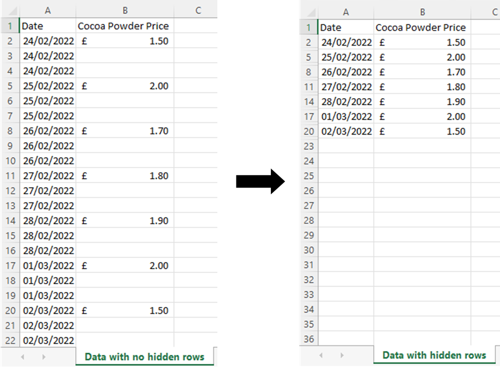
- This will hide all the rows (as shown in the screenshot below)
- Now you can select the range of cells for creating your chart and use F11 key to create it
The video below goes through how to hide the rows seen in the spreadsheet attached here (clicking here will download a copy to your computer so you can try it out!). We hope that you find the video useful and enjoy learning about it!
Take a look below at the video to find out more!
We hope you liked this hint and tip on the creating a chart from hidden rows in Excel, why not take a look at our previous one on aligning and sizing shapes in PowerPoint?