
Nested VLOOKUPs in Excel – using a step-by-step guide to learn and perfect the skill of using them in a spreadsheet
![]() This week’s hint and tip is on nested VLOOKUPs in Excel. Nesting formulas allow you to push the formulas capabilities more and can also help if the data you are matching doesn’t have a simple straightforward match to one table of data. We cover nested VLOOKUPs in our Master Class Excel Bronze training course but as they are so popular, we decided to do a hint and tip on it too. We are going to go through it now below.
This week’s hint and tip is on nested VLOOKUPs in Excel. Nesting formulas allow you to push the formulas capabilities more and can also help if the data you are matching doesn’t have a simple straightforward match to one table of data. We cover nested VLOOKUPs in our Master Class Excel Bronze training course but as they are so popular, we decided to do a hint and tip on it too. We are going to go through it now below.
What is a nested VLOOKUP?
A Nested VLOOKUP, also known as a ‘VLOOKUP within a VLOOKUP’, is an advanced Excel technique that allows you to search for information in multiple layers of data. It allows you to take a simple VLOOKUP and stretch its power and usefulness further!
When Should You Use Nested VLOOKUPs?
Nested VLOOKUPs are incredibly useful when you have complex spreadsheets, such as multi-level tables or databases. They allow you to find information that doesn’t always directly match from the value you are looking up to one table of data. Some examples of how they can be used are:
- Employee Salary Lookup: Finding the salary of an employee based on their department and job title
- Inventory Management: Retrieving the quantity of a specific product in a particular warehouse
- Employee Cost for a Job: Calculating the cost of an employees time on a job based on the hours worked and their hourly rate
How to Build a Nested VLOOKUP
Here’s a simplified example to get you started:
Let’s say you have an Excel workbook with three sheets: Sales, Prices and Products. In the Sales sheet, you want to find the total cost of a product based on the product’s ID and the individual price.
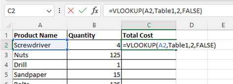
- Step 1: Use the first VLOOKUP to find the product’s ID based on its name:
=VLOOKUP(A2, Table1, 2, FALSE)
In this formula, A2 is the product name, Table1 is the named range containing the product data, and 2 is the column number with the product ID.
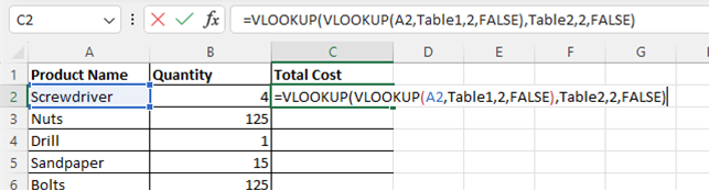
- Step 2: Use the second VLOOKUP to find the price based on the product ID and the year:
=VLOOKUP(VLOOKUP(A2, Table1, 2, FALSE), Table2, 2, FALSE)
In this formula, the inner VLOOKUP retrieves the product ID, and the outer VLOOKUP uses it to find the individual price in the “Prices” sheet.
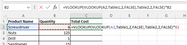
- Finally once you have done the nested VLOOKUP, you need to times all of this by the quantity cell to work out the Total Cost.
Tips for Success:
- Always set the last argument of your VLOOKUP functions to FALSE for exact matches
- Ensure consistent data formatting and structure in both sheets
- Debug your nested VLOOKUPs step by step to catch errors
- Work ‘inside out’, this means your first VLOOKUP then becomes your lookup value for your second VLOOKUP
With the ability to navigate through multiple layers of data, nested VLOOKUPs empower you to unlock the full potential of your Excel skills. Whether you’re managing finances or analysing data, mastering this advanced technique will make you an Excel superstar.
Level up your Excel game today and embrace the magic of nested VLOOKUPs!
Worked example video
The video below shows you how you can use this feature in the spreadsheet attached here. (clicking here will download a copy to your computer so you can try it out!). We hope that you find the video useful and enjoy learning about it!
Take a look below at the video to find out more and then try it out on your own computer!
We hope you have enjoyed this hint and tip on Nested VLOOKUPs in Excel. Why not take a look at our previous video hint and tip on VLOOKUPS in your Excel spreadsheets?